Closure phase errors
This example demonstrates how to estimate the root mean squared error in closure phase induced by scattering. The python script covers:
- Scattering an image
- Generating multiple instances of the screen
- Generating uv samples for closure phase calculations
- Calculating closure phases for an image including Earth rotation.
- Calculating the rms closure phase error induced by scattering.
Closure phases are useful quantities for studying asymmetry when your data has large station-specific phase noise. To compute a closure phase you sum the phases over three directed baselines that represent a closed geographic triangle. While these quantities can be rather unintuitive, it is useful to know that for source with rotational symmetry the closure phase is zero. So in the ensemble-average regime, scattering introduces no error in the closure phase. However, for the distortions introduces in the average image will change the closure phase. The error is dependent upon both the source structure and the screen.
First we will load modules and do some basic configuration:
from scatterbrane import Brane,Target,utilities
import numpy as np
import time
from scipy.ndimage import imread
import matplotlib.pyplot as plt
plt.rcParams['image.cmap'] = 'gray_r'
plt.rcParams['image.origin'] = 'lower'

# set up logger
import logging
logging.basicConfig(level=logging.INFO)
logger = logging.getLogger()
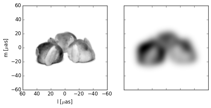
Now we will load our source image and arbitrarily choose its pixel size. Note that I flip the y-axis (axis=0) of the image so that increasing index corresponds to our intuition of up. Scatterbrane assumes that the background level corresponds to 0 so I also invert the color scale.
# import our source image and covert it to gray scale
src_file = 'source_images/640px-Bethmaennchen2.square.jpg'
rgb = imread(src_file)[::-1]
I = 255 - (np.array([0.2989,0.5870,0.1140])[np.newaxis,np.newaxis,:]*rgb).sum(axis=-1)
I = I*np.pi/I.sum()

# and smooth image
I = utilities.smoothImage(I,1.,8.)

# make up some scale for our image. Let's have it span 120 uas.
wavelength=1e-3
FOV = 120.
dx = FOV/I.shape[0]
Our source image and blurred by Gaussian with a full width at half maximum of 10 microarcseconds:
We’ll initialize the scattering screen and the observing parameters for calculating closure phases:
# initialize the scattering screen @ 1mm
b = Brane(I,dx,wavelength=1.e-3,nphi=2**13)

# initialize Target object for calculating visibilities and uv samples
sgra = Target(wavelength=1.e-3)
# calculate uv samples for our closure phase triangle and on the source image
site_triangle = ["SMA","ALMA","LMT"]
(uv,hr) = sgra.generateTriangleTracks(sgra.sites(site_triangle),times=(0.,24.,int(24.*60./2.)),return_hour=True)

# closure phases for the source image
CP_src = sgra.calculateCP(b.isrc,b.dx,uv)
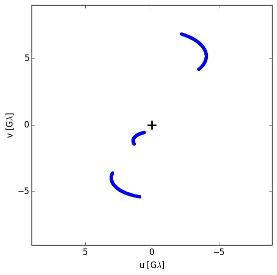
uv is a numpy array with the individual (u,v) pairs separated by 2 minutes. Our closure phase triangle has been set as the SMT, ALMA, and LMT observatories.
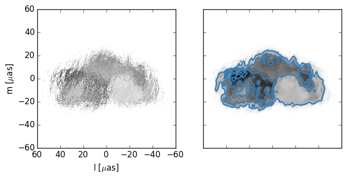
Now we will calculat the closure phaes for a bunch of scattered images using a different phase screen each time. I set the number to take about 10 minutes.
def one_sim(i):
    ''' helper function to run one simulation '''
    global sgra,b,CP
    b.generatePhases()
    b.scatter()
    CP.append(sgra.calculateCP(b.iss,b.dx,uv))

# initialize list
CP = []

# estimate time for one simulation
tic = time.time()
one_sim(0)

# run enough to take about 10 minutes
num_sim = int(10*60. / (time.time()-tic))
logger.info('running {0:g} simulations'.format(num_sim))
tic = time.time()
for i in xrange(1,num_sim):
    one_sim(i)
CP = np.asarray(CP)
logger.info('took {0:g}s'.format(time.time()-tic))
Here is the result for one simulation:
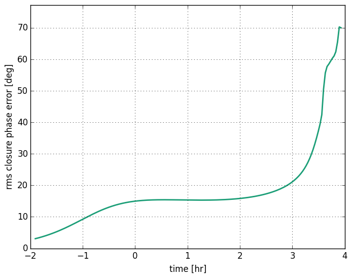
Using our results we can calculate the rms error:
# calculate rms error of closure phase array (CP)
wrapdiff = lambda angle1,angle2: np.angle(np.exp(1j*angle1)/np.exp(1j*angle2))
rms_CP = np.sqrt(np.mean((wrapdiff(CP,CP_src[np.newaxis,:]))**2,axis=0))
and plot it: